Transcribing Piano Rolls, the Pythonic Way

In this post I use Fourier transforms to revive a forgotten Gershwin piano piece.

Piano rolls are these rolls of perforated paper that you feed to the saloon’s mechanical piano. They have been very popular until the 1950s, and the piano roll repertory counts thousands of arrangements (some by greatest names of jazz) which have never been published in any other form.

Here is Limehouse Nights, played circa 1918 by a 20-year-old George Gershwin:

It is cool, it is public domain music, and I want to play it. But like for so many other rolls, there is no published sheet music.

Fortunately, someone else filmed the same performance with a focus on the roll:

In this post I show how to turn that video into playable sheet music with the help of a few lines of Python. At the end I provide the sheet music, a human rendition, and a Python package that implements the method (and can also be used to transcribe from MIDI files).

Downloading the video

You can download the video from Youtube using youtube-dl in a terminal:

youtube-dl wMsEbYCh7yY -o limehouse_nights.mp4

Step 1: Segmentation of the roll

In each frame of the video we will focus on a well-located line of pixels:

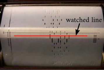
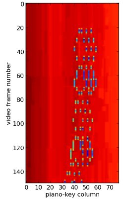
By extracting this line from each video frame and stacking the obtained lines on one another we can reconstitute an approximate scan of the piano roll:

# Required Python modules
from moviepy.editor import VideoFileClip # for video processing
from pylab import * # for mathematics/plotting

# load the video, keep the clip between t=2s and t= 30s
video = VideoFileClip('./limehouse_nights.mp4').subclip(2,30)


# extract the focus lines in the different frames, stack them.
roll_picture = vstack([frame[[156],58:478]
                       for frame in video.iter_frames()])

imshow( roll_picture ) # display the obtained picture

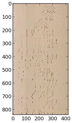
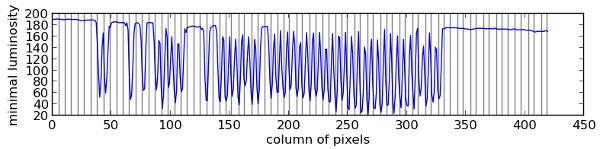
We can see that the holes are placed along columns. Each of these columns corresponds to one key of the piano. A possible way to find the x-coordinates of these columns in the picture is to look at the minimal luminosity of each column of pixels:

roll_greyscale = roll_picture.mean(axis=2) # RGB to grey
luminosity_per_column = roll_greyscale.min(axis=0)

plot( luminosity_per_column)
xlabel('column of pixels (x-index)')
ylabel('minimal luminosity')

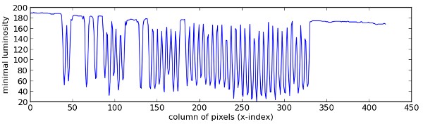
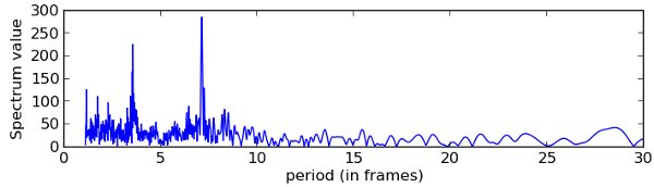
Holes are low-luminosity zones in the picture, therefore the x-coordinates with lower luminosity in the curve above indicate hole-columns. They are not equally spaced because some piano keys are not used in this piece, but there is clearly a dominant period, which we will find by looking at the frequency spectrum of the curve.

We compute that spectrum using a continuous Fourier transform. The peaks in the spectrum below mean that a periodic pattern is present in the curve:

n_lines, n_columns = roll_greyscale.shape
tt = arange(n_columns) # 0,1,2,3,4... n_columns
lum0 = luminosity_per_column - luminosity_per_column.mean()

def fourier_transform(signal, period, tt):
    """ See http://en.wikipedia.org/wiki/Fourier_transform
    I could also have used Numpy's fft.
    """
    f = lambda func : (signal*func(2*pi*tt/period)).sum()
    return f(cos)+ 1j*f(sin)

widths = arange(.1,20,.01)
transform = array([ fourier_transform(lum0,w,tt)
                    for w in widths])

plot(widths, abs(transform))
xlabel("Period (in number of pixels)")
ylabel("Spectrum value")

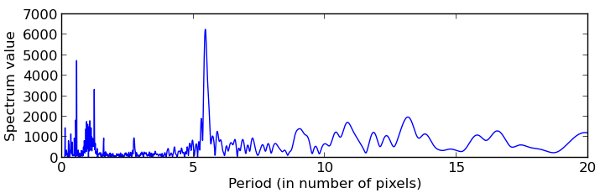
The higher peak of the spectrum indicates a period of x=5.46 pixels, and this is indeed the distance in pixels between two hole-columns. This, plus the phase of the spectrum in this point, gives us the coordinates of the centers of the hole-columns (vertical lines below).

# The maximum the transform indicates the holes' width
optimal_i = argmax(abs(transform))
hole_width = widths[optimal_i]
offset = angle(transform[optimal_i]) +hole_width/2 # to be revised.

keys_positions = arange(offset, n_columns, hole_width)
keys_positions = np.round(keys_positions).astype(int)

plot(luminosity_per_column)
for h in keys_positions:
    axvline(h, c='k', alpha=0.5)
xlabel('column of pixels')
ylabel('minimal luminosity')

We can now reduce our image of the piano roll to keep only one pixel per hole-column. In the resulting picture, one column gives the time profile of one key in the piano: when it is pressed, and when it is released.

keys_greyscale = roll_greyscale[:, keys_positions]

imshow(keys_greyscale[0:150])
xlabel('piano-key column')
ylabel('video frame number')

To reconstitute the sheet music the most important is to know when a key is pressed, not really when it is released. So we will look for the beginning of the holes, i.e. pixels that present a hole, while the pixel just above them doesn’t.

# we threshold the picture to separate the pixels
# into 'hole' and 'no-hole'
key_pressed = keys_greyscale < 0.8*keys_greyscale.max()
# We look at the differences between consecutive lines
key_changes =  diff(key_pressed.astype(int), axis=0)

imshow(key_changes)

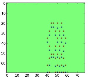
This worked quite well: in the picture above red dots indicate key strikes and blue dots indicate key releases. Let us gather all the key strikes in a list.

Ly, Lx = key_changes.shape
keys_strikes = [(i, j) # (column number, strike time)
                for i in range(Ly)
                for j in range(Lx)
                if key_changes[i, j] == 1]

Step 2: Finding the pitch

We know that the columns correspond to piano keys. They are sorted left to right from the lowest to the highest note. But which column corresponds to the C4 (the middle C)?

I cheated a little and I looked at the first video (the one where you can see the piano keyboard) to see which notes were pressed in the first chords. I concluded that C4 is represented by column 34.

From now on I would like the musical notes C4, C#4, D4… to be coded by their respective numbers in the MIDI norm: 60, 61, 62… So I will transpose my list of key strikes by adding 26 to each note.

transpose = 26
keys_strikes = [(t, key+transpose)
                for t, key in keys_strikes ]

Step 3: Quantization of the notes

We have a list of notes with the time (or frame) at which they are played. We will now determine which notes are quarters, which are eights, etc. This operation is equivalent to finding the tempo of the piece. Let us first have a look at the times at which the the piano keys are striken:

strike_times = (key_changes == 1).sum(axis=1)
plot(strike_times)
xlabel('frame number'); ylabel('number of keys hit')

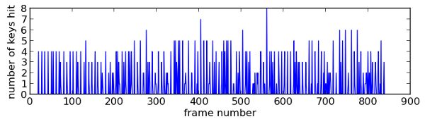
We observe regularly-spaced peaks corresponding to chords (several notes striken together). In this kind of music, chords are mainly played on the beat. Therefore, computing the main period in the graph above will give us the duration of a beat (or quarter). Let us have a look at the spectrum.

tt = arange(len(strike_times))
durations = arange(1.1,30,.02) # avoid 1.0
transform = array([fourier_transform(strike_times,d, tt)
                    for d in durations] )
optimal_i = argmax(abs(transform))
quarter_duration = durations[optimal_i]

plot(durations, abs(transform))
xlabel('period (in frames)'); ylabel('Spectrum value')

The higher peak indicates that a quarter has a duration corresponding to 7.1 frames of the video. Just for info, we can estimate the tempo of the piece with

tempo = int(video.fps * 60.0/quarter_duration) # we find 252.

We will now separate the hands. Let us keep things simple and say that the left hand takes all the notes below the middle C.

C4 = 60
left_hand = [(t,key) for (t,key) in keys_strikes if key<C4]
right_hand = [(t,key) for (t,key) in keys_strikes if key>=C4]

Then we quantize the notes of each hand with the following algorithm: compute the time duration $d$ between a note and the previous note, and compare $d$ to the duration $Q$ of the quarter:

If $d < Q/4$, consider that the two notes belong to the same chord.
Else, if $Q/4 \leq d < 3Q/4$ , consider that the previous note was an eighth.
Else, if $ 3Q/4 \leq d < 5Q/4 $, consider that the previous note was a quarter
etc.

And we treat the notes one after another:

def quantize(keys_strikes, quarter_duration):

    # the result is initialized with one 'empty' note.
    result = [ {'notes':[], 'duration':None, 't_strike':0} ]

    for time, key in keys_strikes:

        # time elapsed since last strike 
        delay = time - result[-1]['t_strike']
        # the next line quantizes that time in eights.
        delay_q = 0.5*int((4.0*delay/quarter_duration+1)/2)

        if (delay_q == 0):# put note in previous chord
            if key not in result[-1]['notes']:
                result[-1]['notes'].append(key)

        else: # this is a 'new' note/chord
            result[-1]['duration'] = delay_q
            result.append( {'notes': [key],
                            'duration': None,
                            't_strike':time} )

    result[-1]['duration'] = 4 # give duration to last note

    if result[0]['notes'] == []:
        result.pop(0) # first note will surely be empty

    return result

left_hand_quantized = quantize(left_hand, quarter_duration)
right_hand__quantized = quantize(right_hand, quarter_duration)

The final data looks like this:

>>> right_hand_q[:4]
#> [{'duration': 1.0, 'notes': [70, 72, 76, 80], 't_strike': 20},
#>  {'duration': 1.0, 'notes': [68, 74, 78, 82], 't_strike': 28},
#>  {'duration': 1.0, 'notes': [66, 76, 80, 84], 't_strike': 35},
#>  {'duration': 1.0, 'notes': [68, 74, 78, 82], 't_strike': 43}]

Step 4: Export to sheet music with Lilypond

Our script’s last task is to convert these lists of quantized notes to a music notation language called Lilypond, which wan be compiled into high-quality sheet music. Some packages like music21 can do that, but it is also fairly easy to program your own converter:

# non-exhaustive lists (but will do for our example)
lilynotes = ['c', 'cis', 'd', 'ees', 'e', 'f',
             'fis', 'g', 'gis', 'a', 'bes', 'b']
lilyoctaves = [',,,',',,',',','',"'", "''", "'''"]
lilydurations = {0.5:'8', 1:'4', 1.5:'4.', 2:'2',
                 3: '2.', 4:'1'}


def midi2lily(note):
    """ converts  60->c, and 61->cis, etc. """
    octave, rank = (note / 12) - 1 , note % 12
    return lilynotes[rank]+lilyoctaves[octave]


def strike2lily(strike):
    """ converts [60,64],1 -> <c e>4 """
    notes, duration =strike['notes'], strike['duration']

    if len(notes) > 1: # chord
        chord = ' '.join(map(midi2lily, sorted(notes)))
        return"< %s >"%chord +lilydurations[duration]
    else:
        return midi2lily(notes[0]) +lilydurations[duration]


def lilyscore(strikes):
    """ converts a python list of srikes into Lilypond """
    return "\n".join(map(strike2lily,strikes))

left_hand_lily = lilyscore(left_hand_quantized)
right_hand_lily = lilyscore(right_hand_quantized)

Then we write this lilyfied sheet music in a file and render the sheet music by calling lilypond as an external program:

filename = "limehouse.ly"

with open(filename, 'w+') as f:
    f.write("\score{\\new Voice{ \\tempo 4=%d"%tempo
            + "\n %s}}"%right_hand_lily)

# render the sheet music by running Lilypond
import os
os.system('lilypond %s'%filename)

The resulting PDF file starts like this (we only asked for the right-hand part):

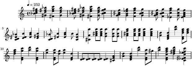
The script has made a pretty good work, all the notes are there with the right pitch and the right duration. If we transcribe the whole piece we will see some mistakes (mostly notes attributed to the wrong hand, and more rarely notes with a wrong duration, wrong pitch, etc.), which have to be corrected, but still it is pretty cool to have these 1500 notes crunched in just a few seconds.

Final result

After 3 hours of editing (with the Lylipond editor Frescobaldi, which I recommend) we come to this playable sheet music (PDF) and I can tease the keyboard like I’m George Gershwin !

Ok, it’s just the first bars - I am still unhappy with my rendition of the rest, it’s a pretty demanding piece.

Since the piece is in the public domain I also put my transcription in the public domain, and placed its lilypond source here on Github (feel free to share/correct/modify it !).

I also wrapped this code into a python package called Unroll which can transcribe from a video of from a midi file (it uses the package music21 for lilypond conversion, and also provides a convenient LilyPond piano template).

from unroll import video2scan, rollscan2keystrikes, KeyStrikes
# just transcribe until t=74s, after this it is a repeat.
scan = video2scan(videofile = "limehouse_nights.mp4",
                  start=2, end=74,
                  focus = lambda im : im[[156],58:478])
keystrikes = rollscan2keystrikes(scan, report=True).transposed(26)
keystrikes.transcribe('test2.ly', quarter_durations =[2,10,0.01])

Oh, and that video of me playing was also made with Python (and my library MoviePy). Here is the script that generated it.

A final word on piano rolls transcription

I have been transcribing rolls as an occasional hobby for years, and I am not the only one: here is another transcriber, and another and yet another. Even Limehouse Nights has apparently been recorded in 1992 but the pianist didn’t publish his transcription.

Most of us transcribe from MIDI files which are made from piano rolls scans (starting from MIDI files is equivalent to starting directly to Step 3, quantization and hands separation). Thousands of MIDI files from rolls scans are available on the internet (like here or here) but not all mechanical piano owners have an appropriate scanner, so there must be thousands of other rolls in private collections which have never been scanned and pushed on the Internet. With this post I wanted to show that just filming piano rolls in action is enough for transcriptions purposes.

del( self )

Eaten by the Python.