Looping GIFs are a very popular form of art on the Web, with two dedicated forums on Reddit (r/perfectloops and r/cinemagraphs) and countless Tumblr pages.
Finding and extracting well-looping segments from a movie requires much attention and patience, and will likely leave you like this in front of your computer:
To make things easier I wrote a Python script which automates the task. This post explains the math behind the algorithm and provides a few examples of use.
We will say that a video segment loops well when its first and last video frames are very similar. A video frame can be represented by a sequence of integers whose values indicate the colors of the image’s pixels. For instance, and give the Red, Green, Blue values of the first pixel, , , define the color of the second pixel, etc.
Given two frames , of a same video, we define the difference between these frames as the sum of the differences between their color values:
We will consider that the two frames are similar when is under some arbitrary threshold .
For what follows, it is important to note that defines a distance between the frames, and can be seen as a generalization of the geometrical distance between two points in a plane:
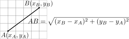
As a consequence has nice mathematical properties which we will use in the next section to speed up computations.
In this section we want to find the times (start and end) of all the well-looping video segments of duration 3 seconds or less in a given video. A simple way to do this is to compare each frame of the movie with all the frames in the previous three seconds. When we find two similar frames (that is, whose distance in under some pre-defined threshold ), we add their corresponding times to our list.
The problem is that this method requires a huge number of frame comparisons (around ten millions in a standard video) which takes hours. So let us see a few tricks to makes computations faster.
Trick 1: use reduced versions of the frames. HD videos frames can have millions of pixels, so computing the distance between them will require millions of operations. When reduced to small (150-pixel-wide) thumbnails these frames are still detailed enough for our purpose, and their distance can be computed much faster (they also take less place in the RAM).
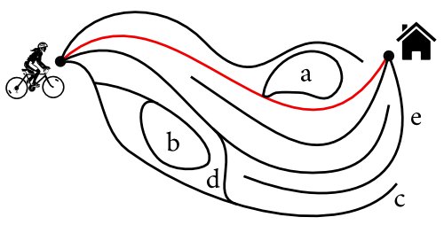
Trick 2: use triangular inequalities. With this very efficient trick we will be able to deduce whether two frames match, without having to compute their distance. Since defines a mathematical distance between two frames, many results from classical geometry apply, and in particular the following inequalities on the lengths of a triangle:
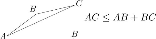
The first inequality tells us that if A is very close to B which in turn is very close to C, then A is also close to C. In terms of video frames, this becomes:
In practice we will use it as follows: if we already know that a frame is very similar to a frame , and that is very similar to another frame , then we do not need to compute to know that and are also very similar.
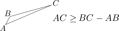
The second inequality tells us that if a point A is very near from B, and B is far from C, then A is also far from C. Or in terms of frames:
If is very similar to , and is different from , then we do not need to compute to know that and are also very different.
Now it gets a little more complicated: we will apply these triangular inequalities to get information on the upper and lower bounds of the distances between frames, which will be updated every time we compute a distance between two frames. For instance, after computing the distance , the upper and lower bounds of , denoted and , can be updated as follows:
If after the update we have , we conclude that and are a good match. And if at some point , we know that and don’t match. If we cannot decide whether and match using this technique, we will eventually need to compute , but then knowing will in turn enable us to update the bounds on another distance, , and so on.
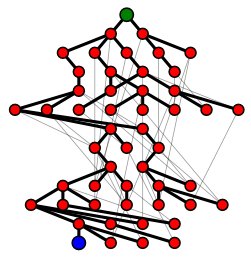
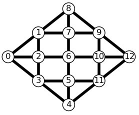
As an illustration, suppose that a video has the following frames in this order:
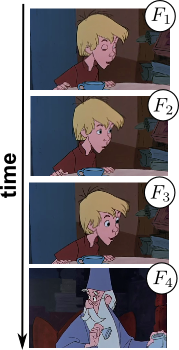
When the algorithm arrives at , it first computes the distance between this frame and and finds that they don’t match. At this point the algorithm has already found thaft is quite similar to and , so it deduces that neither nor match with (and, certainly, neither do the dozen frames before ). In practice, this method avoids computing 80% to 90% of the distances between frames.
Trick 3: use an efficient formula for the distance. When we compute the distance between two frames using the formula from the last section, we need approximately operations: subtractions, products, and additions to obtain the final sum. But the formula for can also be rewritten under this form, known as the law of cosines:
where we used the following notations:
The interesting thing with this expression of is that if we first compute the norm of each frame once, we can obtain the distance between any pair of and simply by computing , which requires only operations and is therefore 50% faster.
Another advantage of computing for each frame is that for two frames and we have
which provides initial values for the upper and lower bounds on the frame distances used in Trick 2:
Final algorithm in pseudo-code. Putting everything together, we obtain the following algorithm:
1 2 3 4 5 6 7 8 9 10 11 12 13 14 15 16 17 18 19 20 21 22 23 24 25 26 |
|
Here is the implementation in Python. The computation time may depend on the quality of the video file, but most movies I tried were processed in circa 20 minutes. Impressive, right, Eugene ?
The algorithm described in the previous section finds all pairs of matching frames, including consecutive frames (which often look very much alike) and frames from still segments (typically, black screens). So we end up with typically a hundred thousand video segments, only a few of which are really interesting, and we must find a way to filter out all the segments we don’t want before extracting GIFs. This filtering operation takes just a few seconds but its success depends greatly on the filtering criteria you use. Here are some examples that work well:
I try to be not too restrictive (to avoid filtering out good segments by accident) so I generally end up with about 200 GIFs, many of them them only midly interesting (blinking eyes and such). The last step is a manual filtering which looks like this:
I implemented this algorithm as a plugin of my Python video library MoviePy. Here is an example script with much details:
1 2 3 4 5 6 7 8 9 10 11 12 13 14 15 16 17 18 19 20 21 22 23 24 25 26 27 28 29 |
|
Here is what be obtain when we try it on Disney’s Snow White:
1 2 3 4 5 6 |
|
Some of these GIFs could be cut better, some are not really interesting (too short), and a few looping segments have been missed. I think the culprits are the parameters in the last filtering step, which could have been tuned better.
As another example, someone recently posted a Youtube video on r/perfectloops and required that it be transformed into a looping GIF. The following script does just that: it downloads the video from Youtube, finds the best times (t1,t2) to cut a looping sequence, and generates a GIF:
1 2 3 4 5 6 7 8 9 10 11 12 13 |
|
With MoviePy you can also post-process your GIFs to add text:
And since you read until there, here is a more advanced trick for you:
The algorithm I presented here is not perfect. It works poorly with low-luminosity clips, and sometimes a slight camera movement or a moving object in the background can prevent a segment from looping. While these segments could be easily corrected by a human, they are more difficult to spot and process with an algorithm.
So my script didn’t completely kill the game, and making looping gifs is still an art. If you have any ideas or remarks on the algorithm, or if you tried it and found some interesting loops in a movie, I’ll be happy to hear about it ! Until then, cheers, and happy GIFing !
]]>MoviePy lets you define custom animations with a function make_frame(t)
, which returns the video frame corresponding to time t
(in seconds):
1 2 3 4 5 6 7 8 9 10 11 12 |
|
In previous posts I used this method to animate vector graphics (with the library Gizeh), and ray-traced 3D scenes (generated by POV-Ray). This post covers the scientific libraries Mayavi, Vispy, Matplotlib, Numpy, and Scikit-image.
Mayavi is a Python module for interactive 3D data visualization with a simple interface. In this first example we animate a surface whose elevation depends on the time t
:
1 2 3 4 5 6 7 8 9 10 11 12 13 14 15 16 17 18 19 20 21 22 |
|
Another example with a wireframe mesh whose coordinates and view angle depend on the time :
1 2 3 4 5 6 7 8 9 10 11 12 13 14 15 16 17 18 19 20 21 22 23 24 25 26 27 28 |
|
As Mayavi relies on the powerful ITK visualization engine it can also process complex datasets. Here is an animation derived from a Mayavi example:
Vispy is another interactive 3D data visualization library, based on OpenGL. As for Mayavi, we first create a figure and a mesh, that we animate with MoviePy.
1 2 3 4 5 6 7 8 9 10 11 12 13 14 15 16 17 18 19 20 21 22 23 24 25 26 27 28 |
|
Here are more advanced examples (derived from the Vispy gallery) where C code snippets are embedded in the Python code to fine-tune the 3D shaders:
The 2D/3D plotting library Matplotlib already has an animation module, but I found that MoviePy produces lighter, better quality videos, while being up to two times faster (not sure why, see here for more details). Here is how you animate Matplotlib with MoviePy:
1 2 3 4 5 6 7 8 9 10 11 12 13 14 15 16 17 18 19 20 21 22 23 24 |
|
Matplotlib has many beautiful themes and works well with numerical modules like Pandas or Scikit-Learn. Let us watch a SVM classifier getting a better understanding of the map as the number of training point increases.
1 2 3 4 5 6 7 8 9 10 11 12 13 14 15 16 17 18 19 20 21 22 23 24 25 26 27 28 29 30 31 32 |
|
Put simply, the background colors tell us where the classifier thinks the black points and white points belong. At the begining it has no real clue, but as more points appear it progressively understands that they are distributed along moon-shaped regions.
If you are working with Numpy arrays (Numpy is the central numerical library in Python), you don’t need any external plotting library, you can feed the arrays directly to MoviePy.
This is well illustrated by this simulation of a zombie outbreak in France (inspired by this blog post by Max Berggren). France is modelled as a grid (Numpy array) on which all the computations for dispersion and infection are done. At regular intervals, a few Numpy operations tranform the grid into a valid RGB image, and send it to MoviePy.
What is better than an animation ? Two animations ! You can take advantage of MoviePy’s video composition capabilities to mix animations from different libraries:
1 2 3 4 5 6 |
|
Or for something more artistic:
1 2 3 4 5 6 7 8 |
|
It may be a tad too flashy, but sometimes you must give your audience something they can tweet.
You can also annotate the animations, which is useful when comparing different filters or algorithms. Let’s display four image transformations from the library Scikit-image:
1 2 3 4 5 6 7 8 9 10 11 12 13 14 15 16 17 18 19 20 21 22 23 24 25 26 |
|
If we replace CompositeVideoClip
and clips_array
by concatenate_videoclips
we get a title-effect type animation:
1 2 3 4 5 6 7 8 9 10 11 12 13 14 15 16 17 18 19 20 21 22 23 24 25 |
|
Finally, MoviePy will be particularly practical when dealing with video data, as it is its first job. For our last example we estimate the size of a growing bacterial population by thresholding the video frames and counting the white pixels. The third panel shows that the population size grows exponentially in time.
I hope to have given you enough recipes to impress your colleagues at your next presentation. Any other library could be animated with MoviePy, as long as its output can be converted to a Numpy array.
Some libraries have their own animation modules, but these are usually a pain to fix and maintain. Thanks to the many users who have tested it in very different contexts, MoviePy seems to have become stable (or people stopped reporting bugs), and can be adapted to many situations. There is still a lot to do, but it would be nice if authors started relying on it for video and GIF rendering, like Pandas and Scikit-Learn rely on Matplotlib for plotting.
For completeness, and because it may better fit your needs, I must mention ImageIO, another Python library with video writing capabilities which focuses on providing a very simple interface to read or write any kind of image, video or volumetric data. For instance you use imwrite()
to write any image, mimwrite()
for any video/GIF, volwrite()
for volumetric data, or simply write()
for streamed data.
Cheers, and happy GIFing !
]]>POV-ray is a popular 3D rendering software which produces photo-realistic scenes like this one:
It may not be as good as Cinema4D or Pixar’s RenderMan, but POV-Ray is free, open-source, and cross-platform. Rendering is launched from the terminal with povray myscene.pov
, where myscene.pov
contains the description of a 3D scene:
1 2 3 4 |
|
While POV-Ray has a very nice and sophisticated scene description language, I wanted to use it together with libraries from the Python world, so I wrote Vapory, a library to render POV-Ray scenes directly from Python, like this:
1 2 3 4 5 6 7 8 9 |
|
This script simply generates a scene.pov
file (hat tip this script by Simon Burton) and then sends the file to POV-Ray for rendering. Vapory can also pipe the resulting image back to Python, and has a few additional features to make it easy to use in an IPython Notebook.
We first create a scene where the positions of the objects depend on the time :
1 2 3 4 5 6 7 8 9 10 11 12 13 |
|
Then we animate this scene with MoviePy:
1 2 3 4 5 6 |
|
Note that one can also make basic animations directly with POV-Ray. But since we use Python we can use its image processing libraries for post-processing. As an example, let us use Scikit-image’s sobel filter to obtain a nice geometry animation
1 2 3 4 5 6 7 8 9 10 11 12 13 14 |
|
The contours look pretty nice because POV-Ray uses exact formulas to render geometrical objects (contrary to libraries like ITK or OpenGL, which rely on triangular meshes). With a few more lines we can mix the two animations to create a cel-shading effect:
1 2 3 4 5 6 |
|
Since we are playing around with MoviePy, let’s embed an actual movie in a 3D scene:
We start with a basic scene:
1 2 3 4 5 6 7 8 9 10 11 12 13 14 15 16 17 18 |
|
To this scene we will add a flat box (our theater screen), and for each frame of the movie we will make a PNG image file that will be used by POV-Ray as the texture of our flat box.
1 2 3 4 5 6 7 8 9 10 11 12 13 14 15 16 17 18 19 20 21 |
|
This 25-seconds clip takes 150 minutes to generate (!!!) which may be due to the good resolution settings, numerous light reflexions in the balls and the ground, and the complex texture of the screen.
In this exemple we write “VAPORY” using 240 bricks:
First, we generate an image of the white-on-black text “VAPORY”. Many libraries can do that, here we use ImageMagick through MoviePy:
1 2 3 4 5 |
|
Here is the result:
We then get the coordinates of the non-black pixels is this image, and use them to place the bricks in the 3D scene, with small random variations around the depth-axis:
1 2 3 4 5 6 7 8 9 10 11 12 13 14 15 16 17 18 19 20 21 |
|
Python as many nice scientific and engineering libraries that could benefit from a photorealistic rendering engine. Here I simulated the cube trajectories with PyODE (a Python binding of the physics engine ODE), and fed the results to Vapory and MoviePy for rendering and animation, all in a hundred lines.
In a previous post I talked about how piano rolls can be scanned and turned into MIDI files (which are some sort of electronic sheet music). Here is a 1997 student project where they used such a MIDI file to animate a 3D piano programatically:
Python has now all the libraries for such a project: we can parse the MIDI file with the package mido, and render the piano keyboard with Vapory. We can convert the MIDI file to an MP3 audio file by calling FluidSynth externally and finally use MoviePy to animate everything and incorporate the audio.
Here is Let’s Fall in Love, from a 1933 piano roll arranged by J. Lawrence Cook, and animated with just ~100 lines of code:
I hope to have shown that Python and POV-Ray can do nice things together, all easy-peasy with Vapory. On the longer term, it would be nice if more recent softwares like Blender (which has a huge user community and modern features like GPU acceleration) had proper Python bindings. But apparently this will never happen.
]]>I am a big fan of Dave Whyte’s vector animations, like this one:
It was generated using a special animation language called Processing (here is Dave’s code). While it seems powerful, Processing it is not very elegant in my opinion ; this post shows how to do similar animations using two Python libraries, Gizeh (for the graphics) and MoviePy (for the animations).
Gizeh is a Python library I wrote on top of cairocffi
( a binding of the popular Cairo library) to make it more intuitive. To make a picture with Gizeh you create a surface, draw on it, and export it:
1 2 3 4 5 6 7 8 |
|
We obtain this magnificent Japanese flag:
To make an animation with MoviePy, you write a function make_frame
which, given some time t
, returns the video frame at time t
:
1 2 3 4 5 6 7 8 9 10 |
|
We start with an easy one. In make_frame
we just draw a red circle, whose radius depends on the time t
:
1 2 3 4 5 6 7 8 9 10 11 12 13 14 15 |
|
Now there are more circles, and we start to see the interest of making animations programmatically using for
loops. The useful function polar2cart
transforms polar coordinates (radius, angle) into cartesian coordinates (x,y).
1 2 3 4 5 6 7 8 9 10 11 12 13 14 15 16 17 18 19 20 21 22 23 |
|
Here we fill the circles with a slightly excentred radial gradient to give and impression of volume. The colors, initial positions and centers of rotations of the circles are chosen randomly at the beginning.
1 2 3 4 5 6 7 8 9 10 11 12 13 14 15 16 17 18 19 20 21 22 23 24 25 26 27 |
|
The shadow is done using a circle with radial fading black gradient whose intensity diminishes when the ball is higher, for more realism (?). The shadow is then squeezed vertically using scale(r,r/2)
, so that its width is twice its height.
1 2 3 4 5 6 7 8 9 10 11 12 13 14 15 16 17 18 19 20 21 22 23 24 25 26 27 28 29 30 31 32 |
|
This is a derivative of the Dave Whyte animation shown in the introduction. It is made of stacked circles moving towards the picture’s border, with carefully chosen sizes, starting times, and colors (I say carefully chosen because it took me a few dozens random tries). The black around the picture is simply a big circle with no fill and a very very thick black border.
1 2 3 4 5 6 7 8 9 10 11 12 13 14 15 16 17 18 19 20 21 22 23 24 25 26 27 28 29 30 31 32 33 |
|
You can draw more than circles ! And you can group different elements so that they will move together (here, a letter and a pentagon).
1 2 3 4 5 6 7 8 9 10 11 12 13 14 15 16 17 18 19 20 21 22 23 24 25 |
|
We start with just a triangle. By rotating this triangle three time we obtain four triangles which fit nicely into a square. Then we copy this square following a checkerboard pattern. Finally we do the same with another color to fill the missing tiles. Now, if the original triangle is rotated, all the triangles on the picture will also be rotated.
1 2 3 4 5 6 7 8 9 10 11 12 13 14 15 16 17 18 19 20 21 22 23 24 25 26 27 28 29 30 31 32 33 34 |
|
A nice thing to do with vector graphics is fractals. We first build a ying-yang, then we use this ying-yang as the dots of a bigger ying-yang, and we use the bigger ying-yang as the dots of an even bigger ying yang etc. In the end we go one level deep into the imbricated ying-yangs, and we start zooming.
1 2 3 4 5 6 7 8 9 10 11 12 13 14 15 16 17 18 19 20 21 22 23 24 25 26 27 28 29 30 31 32 33 34 35 36 |
|
That one is inspired by this Dave Whyte animation. We draw white-filled circles, each of these being almost completely transparent so that they only add 1 to the value of the pixels that they cover. Pixels with an even value, which are the pixels covered by an even number of circles, are then painted white, while the others will be black. To complexify and have a nicely-looping animation, we draw two circles in each direction, one being a time-shifted version of the other.
1 2 3 4 5 6 7 8 9 10 11 12 13 14 15 16 17 18 19 20 |
|
A pentagon made of rotating squares ! Interestingly, making the squares rotate the other direction creates a very different-looking animation. The squares are placed according to this polar equation.
The difficulty in this animation is that the last square drawn will necessarily be on top of all the others, and not, as it should be, below the first square ! The solution is to draw each frame twice. The first time, we draw the squares starting from the right, so that the faulty square will also be on the right, and we only keep the left part of that picture. The second time we start drawing the squares from the left, so that the faulty square is on the left, and we keep the right part. By assembling the two valid parts we reconstitute a valid picture.
1 2 3 4 5 6 7 8 9 10 11 12 13 14 15 16 17 18 19 20 21 22 23 24 25 26 27 28 29 30 |
|
A nice advantage of combining Gizeh with MoviePy is that you can read actual video files (or gifs) and use the frames to fill shapes drawn with Gizeh.
We will use this video from the Blender Foundation (it’s under a Creative Common licence). Since you have read until there I’ll show you a little unrelated trick: at 4:32 the rabbit is jumping rope, so there is a potential for a well-looping GIF. We open the video around 4:32, and let MoviePy automatically decide where to cut to have the best-looping GIF possible:
1 2 3 4 5 6 |
|
Now we can feed the frames of this GIF to Gizeh, using MoviePy’s clip.fl(some_filter)
, which means “I want a new clip made by transforming the frames of the current clip with some_filter”.
1 2 3 4 5 6 7 8 9 10 11 12 13 14 15 16 17 18 19 20 21 22 23 24 25 |
|
Finally, this function adds a zoom on some part of the video.
1 2 3 4 5 6 7 8 9 10 11 12 13 14 15 16 17 18 19 20 21 22 23 24 25 26 27 28 29 30 31 32 |
|
I hope I have convinced you that Python is a nice language for making vector animations. If you give it a try, let me know of any difficulty you may meet installing or using MoviePy and Gizeh. And any feedback, improvement ideas, commits, etc. are also very appreciated.
]]>Python modules to interact with Twitter, like tweepy, python-twitter, twitter, or twython, all depend on the Twitter API, which makes them a little complicated to use: you must open a Twitter account, register at dev.twitter.com, open a new application there, and at each connection dance with the OAuth.
If you just want to read the lattest tweets of some Twitter user, instead of using these libraries, you can simply parse the HTML of that user’s Twitter page:
1 2 3 4 5 6 7 8 9 10 11 12 13 14 15 16 17 18 19 |
|
Let us try it on John D. Cook:
1
|
|
1 2 |
|
As an application, here is a script that watches my (useless) Twitter page every 20 seconds, and each time I tweet something like cmd: my_command
it executes my_command
in a terminal:
1 2 3 4 5 6 7 8 9 10 11 12 |
|
I can now tweet-control, from my smartphone, any computer that is running this script. If I tweet cmd: firefox
the computer will open firefox, if I tweet cmd: echo "Hello"
it will print Hello in the terminal, etc.
If you want more, I wrote Twittcher, a small Python module which doesn’t depend on the Twitter API, to make bots that watch search results or user pages and react to the tweets they find.
For instance this script checks the search results for chocolate milk every 20 seconds, and sends all the new tweets (with date, username, and link) to my mail box.
1 2 3 4 5 6 7 8 |
|
Just run that script all day on your computer (or rather on your Raspberry Pi) and you will be updated every time someone drinks chocolate milk and feels the urge to tweet about it (which is very often).
]]>In this post we will make a video summary of this soccer game, using the fact that supporters (and commentators) tend to be louder when something interesting happens.
The next lines open the video file with Python and compute the audio volume of each second of the match:
1 2 3 4 5 6 7 |
|
If we plot the obtained volumes we see that each goal is followed by a few seconds of loudness:
It is much clearer if we compute the average volumes over periods of 10 seconds:
1 2 |
|
The five higher peaks in the above graph give us the times of the five goals of the game, but other peaks may also indicate interesting events. In the next lines, we select the times of the 10% highest peaks:
1 2 3 4 5 |
|
As a refinement, we regroup the times that are less than one minute apart, as they certainly correspond to the same event:
1 2 3 4 5 6 7 |
|
Now final_times
contains the times (in seconds) of 21 events, from which we can cut our video. For each event we will start five seconds before its time and stop five seconds after :
1 2 3 |
|
We obtain the following 3:30 video summary (sorry for the external links, these videos can’t be embedded).
Nicely enough, the same 25 lines of code can be used to cut this other summary of this other match. The limitations of the method appear in yet another summary which only captured 8 out of the 9 goals of the match, one or two being badly cut. The algorithm can be confused by broadcasters which make lots of replays or lower the sound of the crowd after goals, and it may miscut some goals on penalties, because the crowd starts whistling long before the shoot. So large-scale applications would require a less naive model.
If you want to try it at home, here is the whole script. It would be interesting to see how the method works on other sports, or how it could be generalized to other uses, like spotting action scenes in movies.
]]>This week Sam Lavigne wrote a very entertaining blog post introducing Videogrep, a Python script that searches through dialog in videos (using the associated subtitles file), selects scenes (for instance all scenes containing a given word), and cuts together a new video.
The script on Github implements many tweaks and goodies (such as working on multiple files, identifying complex patterns, etc.). In this post I present the code for a minimal videogreper in Python and attempt to refine cuts to get scenes containing whole sentences or single words.
A good place to find public domain videos with subtitles is the White House channel on Youtube. In what follows I will be working on the 2012 State Of The Union Address:
To get both the video and the subtitles you can use youtube-dl in a terminal:
1
|
|
This downloads a video file state.mp4
and a text file state.en.srt
indicating the subtitles as follows:
1 2 3 4 5 6 7 8 |
|
This file can be easily parsed in Python to get a list of elements of the form ([t_start,t_end], text_block)
:
1 2 3 4 5 6 7 8 9 10 11 12 13 14 15 16 17 18 19 20 21 22 23 |
|
1 2 3 |
|
Let us have a look at the most common words in the speech:
1 2 3 4 5 |
|
1 2 3 |
|
Seems like the word “should” has been pronounced a lot. Let us find the times of all the subtitle blocks in which it appears:
1 2 |
|
Now we cut and put together all these scenes using MoviePy:
1 2 3 4 5 6 7 8 9 10 11 |
|
Here is the result:
It is promising, but in some scenes we don’t get to know exactly what should be done, which is frustrating. In the next section we add a little content-awareness to get more relevant cuts.
We now want to cut together all the sentences containing the word “should”. We first explore the whole text looking for sentences containing that word, then we find the subtitle blocks corresponding to the start and end of each sentence, and we cut the video file accordingly.
1 2 3 4 5 6 7 8 9 10 11 12 13 14 15 16 17 |
|
It’s much better:
Note that with just a little more code you could achieve much more. In Videogrep the author uses the Python package pattern
to look for advanced phrase constructions, such as all phrases of the form gerund-determiner-adjective-noun.
Let us take a step in the other direction and see if it is possible to automatically cut a scene with exactly one word or expression, and as little possible of the words around it. Consider the following subtitle block:
1 2 |
|
We can roughly evaluate that the word “We” will be pronounced in the first quarter of the time span (from 3:20.1 to 3:20.85), “can” in the second quarter (from 3:20.85 to 3:21.6), etc. Following this reasoning, here is a function that finds the exact times using the relative position of the characters in the subtitles blocks:
1 2 3 4 5 6 7 8 |
|
Let us try it on “Americans”:
1
|
|
At least some of the cuts worked properly. If we use much-pronounced words we may find at least one correct cut for each of them and we can build a whole sentence:
1 2 3 4 5 6 7 |
|
Wow ! That seemed so real, and it almost made sense. From there the cuts could be refined by hand, but the script did most of the work and surely deserved, if not a Nobel Peace Prize, fourteen minutes of applause:
1 2 3 |
|
I just finished this mix of 60 covers of the Cup Song, entirely edited using this Python script !
The code uses extensively MoviePy, a video editing library I wrote to automatize simple tasks such as title insertions, concatenations, transitions, etc. With this video I hope to show that MoviePy is becoming mature, and that it can be more than just a FFMPEG wrapper or a GIF editor.
]]>For some time now I have been designing labyrinths based on traffic lights, like this one:
I call these Viennese mazes (long story) and since I couldn’t find anything similar on the Web, I assume that this is something new. Here are some more with other shapes, and their solutions.
These mazes are very difficult to design by hand, and this post is about how to ask your computer to do the work for you. We will see what a good Viennese maze is made of, and how to generate one using a simple evolutionary algorithm.
My first intention with Viennese mazes was to make dynamic mazes, with moving walls. But under each Viennese maze there is actually a standard, old-school labyrinth.
To see this we must think in terms of states. A state describes where you are in the maze, and determines where you can go from there. In the maze above, state (c,1,a) means “I am in (c), I have passed 1 traffic light until then, and just before that I was in (a)”. From this state you cannot reach (d) as the light in this street has turned red, and you cannot reach (a) because you just came from here. But you can move to (b) or (g), that is, to state (b,2,c) or state (g,2,c). Note that states such as (c,1,a), (c,4,a), and (c,7,a) are actually the same state, because afer three moves all traffic lights come back to their original position. So there will always be a finite number of states in a Viennese maze.
If we draw a map of all (reachable) states and their connexions we obtain the following states graph :
The green node marks the starting point, while the blue node is a reunion of all states corresponding to the goal (m). The nodes on the $i$-th line from the top can be reached in $i$ moves but no less, thick lines go downwards and thin lines go upwards.
This graph looks like a classical labyrinth, with crossroads, dead ends, loops… at one glance it gives an idea of the complexity and interestingness of the original Viennese maze. Therefore, we will consider that a good Viennese maze is a maze whose states graph makes a good labyrinth.
Here is an illustration of a few criteria which make a labyrinth insteresting :
For the computer to be able to compare mazes and identify the most interesting ones we define scores which will quantify how well each of the criteria 1,2,3, are fullfilled by a given maze. For instance
The final score of a Viennese maze is given by the product
where the exponents reflect the relative importance that we decide to attach to each criterion.
Evaluating this score on the states graph of a Viennese maze is easy: the existence and uniqueness of a solution can be checked using a simple-path-finding algorithm. Dead-ends are simply the nodes of the states graph with no descendents, and the loops of the maze correspond to the thin edges. The states graph itself and its different lines of nodes can be easily computed using Dijkstra’s efficient algorithm to find minimal paths between the start and the different states. The current Python implementation, relying on the Networkx package, enable to evaluate on the order of 1000 mazes per second (depending on their complexity).
Now that we have defined how to score a Viennese maze, we will provide the computer with an uncolored canvas, and we will ask for a coloring (initial color of each traffic light) of this canvas that produces the best score possible :
There are $3^{24}$ (almost three hundred billion) ways of coloring the 24 streets on this canvas, and considering all of them would be too long. But a great many of these colorings make interesting mazes, so we can just look semi-randomly for some of these.
An effective way to do so is to first colorize the canvas in a completely random way, then improve the coloring by repeating the following steps:
Here is a maze being optimized following this mutation/selection procedure (over 24000 mazes were generated, only the successive improvements are shown):
This algorithm can be refined using annealing (in which you first evaluate many different mazes before refining the search around the best one), or any fancier search strategy such as genetic algorithms, ant colonies… What works best is still an open question.
If you want to try and make your own Viennese mazes (using for instance you district as a canvas), I wrote a Python package called vmfactory which implements all the steps discussed above. It can generate two variants of Viennese mazes: one where passing through the same light twice in a row is forbidden, and one where it isn’t (algorithmically, the only difference is the way the states graph is computed).
In the following example, we generate a squared canvas, we initialize a maze with random colors, optimize it, and generate a report (maze/graph/solution):
1 2 3 4 5 6 7 8 9 |
|
The package is based on Networkx, Numpy and Matplotlib. The code is rather short (most of it serves to draw fancy graphs !), and modular : you can easily change the rules, change the way the score is computed, change the optimization procedure, or the way the reports are drawn.
Thank you for reading until there, and happy mazing !
]]>A sound can be encoded as an array (or list) of values, like this:
To make this sound play twice faster, we remove every second value in the array:
By doing so we didn’t only halved the sound’s duration, we also doubled its frequency, making it higher-pitched than the original.
If on the contrary we repeat each value of the array twice, we produce a sound that is slower, with a longer period, and therefore lower-pitched:
Here is a simple Python function that can change the speed of a sound by any factor:
1 2 3 4 5 6 7 |
|
What is more difficult to do is to change the duration of a sound while preserving its pitch (sound stretching), or change the pitch of a sound while preserving its duration (pitch shifting).
Sound stretching can be done using the classical phase vocoder method. You first break the sound into overlapping bits, and you rearrange these bits so that they will overlap even more (if you want to shorten the sound) or less (if you want to stretch the sound), like in this figure:
The difficulty is that the reorganized bits can interfer badly with one another, and some phase-transformation is necessary so that this won’t happen. Here is the Python code, freely rewritten from there:
1 2 3 4 5 6 7 8 9 10 11 12 13 14 15 16 17 18 19 20 21 22 23 24 25 26 |
|
Pitch-shifting is easy once you have sound stretching. If you want a higer pitch, you first stretch the sound while conserving the pitch, then you speed up the result, such that the final sound has the same duration as the initial one, but a higher pitch due to the speed change.
Doubling the frequency of a sound increases the pitch of one octave, which is 12 musical semitones. Therefore to increase the pitch by $n$ semitones we must multiply the frequency by a factor $2^{\frac{n}{12}}$:
1 2 3 4 5 |
|
Let us play around with our new pitch-shifter. We first strike a bowl:
Then we create 50 pitch-shifted derivatives of that sound, ranging from the very low to the very high:
1 2 3 4 5 |
|
We will assign each sound to a key of the computer keyboard, following the order in this file, which organizes the keyboard like this:
We simply tell the computer to play the corresponding sound when a key is pressed, and stop the sound when the key is released:
1 2 3 4 5 6 7 8 9 10 11 12 13 14 15 16 17 18 19 20 21 22 23 24 25 26 27 28 29 30 31 32 33 34 |
|
And we have turned our computer into a piano ! Now, to thank you for reading until there, let me play a little turkish song for you:
Here are all the files you need if you want to try this at home. Since not everyone uses Python, I also coded a pianoputer in Javascript/HTML5 (here) but it is very far from good. It would be really great if an experienced HTML5/JS/elm developer improved it, or rewrote it from scratch.
On a more general note, I find that computers have been under-used to produce performance music. I get it that it is easier to use a piano keyboard or record from an instrument directly, but look at what you can do with just a bowl and 60 lines of Python !
Even a cheap computer has so many controls that would make it a proper music station: you can sing to the microphone, make gestures to the webcam, modulate stuff using the mouse, and control the rest from your keyboard. So many ways to express yourself, and there is a Python package for each of them… Any artistic hacker wanting to make steps in that direction ?
]]>Piano rolls are these rolls of perforated paper that you feed to the saloon’s mechanical piano. They have been very popular until the 1950s, and the piano roll repertory counts thousands of arrangements (some by greatest names of jazz) which have never been published in any other form.
Here is Limehouse Nights, played circa 1918 by a 20-year-old George Gershwin:
It is cool, it is public domain music, and I want to play it. But like for so many other rolls, there is no published sheet music.
Fortunately, someone else filmed the same performance with a focus on the roll:
In this post I show how to turn that video into playable sheet music with the help of a few lines of Python. At the end I provide the sheet music, a human rendition, and a Python package that implements the method (and can also be used to transcribe from MIDI files).
You can download the video from Youtube using youtube-dl in a terminal:
1
|
|
In each frame of the video we will focus on a well-located line of pixels:
By extracting this line from each video frame and stacking the obtained lines on one another we can reconstitute an approximate scan of the piano roll:
1 2 3 4 5 6 7 8 9 10 11 12 13 |
|
We can see that the holes are placed along columns. Each of these columns corresponds to one key of the piano. A possible way to find the x-coordinates of these columns in the picture is to look at the minimal luminosity of each column of pixels:
1 2 3 4 5 6 |
|
Holes are low-luminosity zones in the picture, therefore the x-coordinates with lower luminosity in the curve above indicate hole-columns. They are not equally spaced because some piano keys are not used in this piece, but there is clearly a dominant period, which we will find by looking at the frequency spectrum of the curve.
We compute that spectrum using a continuous Fourier transform. The peaks in the spectrum below mean that a periodic pattern is present in the curve:
1 2 3 4 5 6 7 8 9 10 11 12 13 14 15 16 17 18 |
|
The higher peak of the spectrum indicates a period of x=5.46 pixels, and this is indeed the distance in pixels between two hole-columns. This, plus the phase of the spectrum in this point, gives us the coordinates of the centers of the hole-columns (vertical lines below).
1 2 3 4 5 6 7 8 9 10 11 12 13 |
|
We can now reduce our image of the piano roll to keep only one pixel per hole-column. In the resulting picture, one column gives the time profile of one key in the piano: when it is pressed, and when it is released.
1 2 3 4 5 |
|
To reconstitute the sheet music the most important is to know when a key is pressed, not really when it is released. So we will look for the beginning of the holes, i.e. pixels that present a hole, while the pixel just above them doesn’t.
1 2 3 4 5 6 7 |
|
This worked quite well: in the picture above red dots indicate key strikes and blue dots indicate key releases. Let us gather all the key strikes in a list.
1 2 3 4 5 |
|
We know that the columns correspond to piano keys. They are sorted left to right from the lowest to the highest note. But which column corresponds to the C4 (the middle C)?
I cheated a little and I looked at the first video (the one where you can see the piano keyboard) to see which notes were pressed in the first chords. I concluded that C4 is represented by column 34.
From now on I would like the musical notes C4, C#4, D4… to be coded by their respective numbers in the MIDI norm: 60, 61, 62… So I will transpose my list of key strikes by adding 26 to each note.
1 2 3 |
|
We have a list of notes with the time (or frame) at which they are played. We will now determine which notes are quarters, which are eights, etc. This operation is equivalent to finding the tempo of the piece. Let us first have a look at the times at which the the piano keys are striken:
1 2 3 |
|
We observe regularly-spaced peaks corresponding to chords (several notes striken together). In this kind of music, chords are mainly played on the beat. Therefore, computing the main period in the graph above will give us the duration of a beat (or quarter). Let us have a look at the spectrum.
1 2 3 4 5 6 7 8 9 |
|
The higher peak indicates that a quarter has a duration corresponding to 7.1 frames of the video. Just for info, we can estimate the tempo of the piece with
1
|
|
We will now separate the hands. Let us keep things simple and say that the left hand takes all the notes below the middle C.
1 2 3 |
|
Then we quantize the notes of each hand with the following algorithm: compute the time duration $d$ between a note and the previous note, and compare $d$ to the duration $Q$ of the quarter:
And we treat the notes one after another:
1 2 3 4 5 6 7 8 9 10 11 12 13 14 15 16 17 18 19 20 21 22 23 24 25 26 27 28 29 30 31 |
|
The final data looks like this:
>>> right_hand_q[:4]
#> [{'duration': 1.0, 'notes': [70, 72, 76, 80], 't_strike': 20},
#> {'duration': 1.0, 'notes': [68, 74, 78, 82], 't_strike': 28},
#> {'duration': 1.0, 'notes': [66, 76, 80, 84], 't_strike': 35},
#> {'duration': 1.0, 'notes': [68, 74, 78, 82], 't_strike': 43}]
Our script’s last task is to convert these lists of quantized notes to a music notation language called Lilypond, which wan be compiled into high-quality sheet music. Some packages like music21 can do that, but it is also fairly easy to program your own converter:
1 2 3 4 5 6 7 8 9 10 11 12 13 14 15 16 17 18 19 20 21 22 23 24 25 26 27 28 29 30 31 |
|
Then we write this lilyfied sheet music in a file and render the sheet music by calling lilypond as an external program:
1 2 3 4 5 6 7 8 9 |
|
The resulting PDF file starts like this (we only asked for the right-hand part):
The script has made a pretty good work, all the notes are there with the right pitch and the right duration. If we transcribe the whole piece we will see some mistakes (mostly notes attributed to the wrong hand, and more rarely notes with a wrong duration, wrong pitch, etc.), which have to be corrected, but still it is pretty cool to have these 1500 notes crunched in just a few seconds.
After 3 hours of editing (with the Lylipond editor Frescobaldi, which I recommend) we come to this playable sheet music (PDF) and I can tease the keyboard like I’m George Gershwin !
Ok, it’s just the first bars - I am still unhappy with my rendition of the rest, it’s a pretty demanding piece.
Since the piece is in the public domain I also put my transcription in the public domain, and placed its lilypond source here on Github (feel free to share/correct/modify it !).
I also wrapped this code into a python package called Unroll which can transcribe from a video of from a midi file (it uses the package music21 for lilypond conversion, and also provides a convenient LilyPond piano template).
1 2 3 4 5 6 7 |
|
Oh, and that video of me playing was also made with Python (and my library MoviePy). Here is the script that generated it.
I have been transcribing rolls as an occasional hobby for years, and I am not the only one: here is another transcriber, and another and yet another. Even Limehouse Nights has apparently been recorded in 1992 but the pianist didn’t publish his transcription.
Most of us transcribe from MIDI files which are made from piano rolls scans (starting from MIDI files is equivalent to starting directly to Step 3, quantization and hands separation). Thousands of MIDI files from rolls scans are available on the internet (like here or here) but not all mechanical piano owners have an appropriate scanner, so there must be thousands of other rolls in private collections which have never been scanned and pushed on the Internet. With this post I wanted to show that just filming piano rolls in action is enough for transcriptions purposes.
]]>For this demo we will make a few GIFs out of this trailer:
You can download it with this command if you have Youtube-dl installed:
1
|
|
In what follows we import MoviePy, we open the video file, we select the part between 1’22.65 (1 minute 22.65 seconds) and 1’23.2, reduce its size (to 30% of the original) and save it as a GIF:
1 2 3 4 5 6 |
|
For my next GIF I will only keep the center of the screen. If you intend to use MoviePy, note that you can preview a clip with clip.preview()
. During the preview clicking on a pixel will print its position, which is convenient for cropping with precision.
1 2 3 4 5 |
|
Many GIF makers like to freeze some parts of the GIF to reduce the file size and/or focus the attention on one part of the animation.
In the next GIF we freeze the left part of the clip. To do so we take a snapshot of the clip at t=0.2 seconds, we crop this snapshot to only keep the left half, then we make a composite clip which superimposes the cropped snapshot on the original clip:
1 2 3 4 5 6 7 8 9 10 11 12 |
|
This time we will apply a custom mask to the snapshot to specify where it will be transparent (and let the animated part appear) .
1 2 3 4 5 6 7 8 9 10 11 12 13 14 15 16 17 |
|
Surely you have noticed that in the previous GIFs, the end did not always look like the beginning. As a consequence, you could see a disruption every time the animation was restarted. A way to avoid this is to time-symetrize the clip, i.e. to make the clip play once forwards, then once backwards. This way the end of the clip really is the beginning of the clip. This creates a GIF that can loop fluidly, without a real beginning or end.
1 2 3 4 5 6 7 8 9 10 11 12 13 |
|
Ok, this might be a bad example of time symetrization,it makes the snow flakes go upwards in the second half of the animation.
In the next GIF there will be a text clip superimposed on the video clip.
1 2 3 4 5 6 7 8 9 10 11 12 13 14 15 |
|
The following GIF features a lot of snow falling. Therefore it cannot be made loopable using time-symetrization (or you will snow floating upwards !). So we will make this animation loopable by having the beginning of the animation appear progressively (fade in) just before the end of the clip. The montage here is a little complicated, I cannot explain it better than with this picture:
1 2 3 4 5 6 7 8 9 10 11 12 13 14 |
|
The next clip (from the movie Charade) was almost loopable: you can see Carry Grant smiling, then making a funny face, then coming back to normal. The problem is that at the end of the excerpt Cary is not exactly in the same position, and he is not smiling as he was at the beginning. To correct this, we take a snapshot of the first frame and we make it appear progressively at the end. This seems to do the trick.
1 2 3 4 5 6 7 8 9 10 11 12 |
|
Let’s dive further into the scripting madness: we consider this video around 2’16 (edit: not the video I originally used, it was removed by the Youtube user, I add to find another link):
And we will remove the background to make this gif (with transparent background):
The main difficulty was to find what the background of the scene is. To do so, the script gathers a few images in which the little pigs are are different positions (so that every part part of the background is visible on at least several (actually most) of the slides, then it takes the pixel-per-pixel median of these pictures, which gives the background.
1 2 3 4 5 6 7 8 9 10 11 12 13 14 15 16 17 18 19 20 21 22 23 24 25 26 27 28 29 30 31 32 33 34 35 36 37 38 39 40 41 42 43 44 45 46 47 48 49 50 51 52 53 54 55 56 57 58 59 60 61 62 63 64 |
|
Alice just spotted a white rabbit urging to its rabbit hole ! Given the coordinates of the positions A, B, H, of Alice, the rabbit and the hole, as well as the respective speeds $S_A$ and $S_B$ of Alice and the rabbit, say whether Alice can catch the rabbit before it disappears, and give the time and place of the fastest possible interception.
I guess that I am not the first one to solve this but I couldn’t find any simple solution on the internet. The one I am giving here relies on trigonometry, but interestingly it doesn’t require to compute any trigonometrical function !
If sines give you fever, don’t wait for the first sines of fever (uh uh uh), just skip this part, I summarize everything in the next section.
We call C and $t_C$ the location and the time of the catch. It is straightforward that, since we are looking for the fastest catch, Alice’s trajectory towards C must be a straight line. Here is a sketch of the problem:
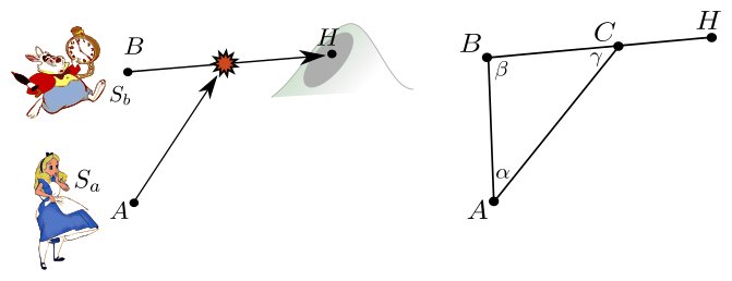
Note that the lengths AC and BC denote the distance run by Alice and the Rabbit until the catch, therefore they verify
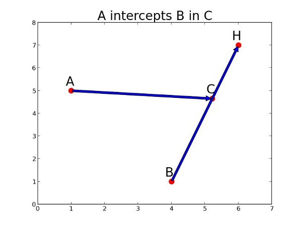
So finding the length BC would answer the problem, as it would tell us whether Alice can catch the rabbit before it reaches the rabbit hole (case $BC<BH$), and would immediately lead to both the location and time of the catch :
To express BC using the coordinates of the points, let us apply the famous Law of Sines to the triangle ABC:
Wich leads to
Now all we have to do is to express $\sin \alpha$ and $\sin \gamma$ in function of the given data. To do so we first compute $\sin(\beta)$, then we express $\sin \alpha$ with $\sin \beta$, and we express $\sin \gamma$ as a function of $\sin \alpha$ and $\sin \beta$.
The value of $\sin \beta$ can be computed from the points coordinates as follows:
Then we use the Law of Sines again, to compute $\sin \alpha$:
This only makes sense, of course, if
If this is not the case we conclude that Alice will never catch the rabbit, which solves the problem.
Finally we use the fact that the angles of a triangle sum to $\pi$ to compute $\sin \gamma$:
We reformulate using the already-copmputed $\sin \alpha$ and $\sin \beta$:
And… we are done, we have everything we need to compute BC and answer the problem.
So here is the short answer to the problem:
Below is a script implementing this technique using Python’s pylab module:
1 2 3 4 5 6 7 8 9 10 11 12 13 14 15 16 17 18 19 20 21 22 23 24 25 26 27 28 29 30 31 32 33 34 |
|
And here it is in action:
1 2 3 4 5 6 7 8 9 10 11 12 13 14 15 16 17 18 19 20 21 22 23 24 25 26 27 28 29 30 31 |
|
Imagine that you have N employees who work side by side in a row. For more conviviality you decide to arrange them in a different order every day, so that after some time each employee has worked besides each of the others at least once. How to do so in a minimal number of days ?
This problem appeared a few weeks ago in the Reddit/Python forum, when someone posted this:
“I think it is good to shuffle the team around. (…) Here is the function that we use to randomize our team making sure that you do not sit next to someone you are already sitting next to [supposing that all are sitting in a row].”.
Stated like this, it is a very simple problem which doesn’t require a complicated algorithm, you just shuffle the order of the previous day as follows, and it will do the trick:
This shuffle can be written in one line of Python:
1 2 |
|
The problem with this shuffling, as someone on Reddit pointed out, is that even if you shuffle a great number of times there is no warranty that everyone will have worked besides everyone else in the end. For instance in the shuffling shown above employees 1 and 8 will never be neighbours. And it seems that you can imagine a shuffling as complicated as you want, there will always be a number of people for which it will fail to create all possible pairs of neighbours !
This leads us to our problem: how to ensure that all possible pairs of neighbours will be created, and in a minimum amount of time ? We will see that there is an optimal strategy. It does NOT use a shuffling, but rather a 120 years old mathematical construction.
If you have N employees, then they can form N(N-1)/2 pairs. Each day you create at most (N-1) new pairs of neighbours by placing the employees on a line. Therefore you will need at least N/2 days to create all possible pairs. This means that you cannot solve the problem in less than N/2 days if N is even, and (N+1)/2 days if n is odd. What we will show is that it is actually possible to solve the problem in N/2 days (for even N) or (N+1)/2 days (for odd N).
In fact we only need to solve the problem for even N, and the solutions for odd N will follow very simply. To see this, suppose that you have an odd number N of employees. If you add one imaginary employee, you come to an even number (N+1) of employees. Suppose that you have found a solution for these (N+1) employees, which means that you have found a series of (N+1)/2 arrangements which form all pairs of neighbours. Then remove the imaginary employee from each of these arrangements. What you obtain is a series of (N+1)/2 arrangements, in which all pairs of the employees 1 to N are formed. In other words, you have solved the problem for N.
This problem can be very well represented using a graph whose nodes are the employees. Each day we add an edge in the graph between each pair of employees which have been neighbours, our goal being to cover all the possible edges of the graph:
Notice how each day you actually trace a path in the graph.
Now our problem has become: given a graph of size N (even), find N/2 paths, each going through each node exactly once, such that they cover all the possible edges of the graph.
And here is a sketch of a solution that will always work:
The first path is a simple pattern 1, N, 2, N-1, etc. and the others are just rotations of the first path. The nice thing with the graph representation is that I can use a simple geometric argument to prove that these paths will cover all the edges: if we place the N nodes of the graph cyclically like in the figures above, the path number K will have edges that make an angle $2K\pi/N$ or $(2K+1)\pi/N$ with the horizontal line. So the different paths have edges of completely different angles. For this reason an edge cannot belong to more than one path. Since there are N/2 paths and each path covers N-1 different edges, the paths cover N(N-1)/2 edges in total, which is all the edges.
This construction of paths may seem simple to some of you, but I couldn’t figure it out on my own, and it is an application of a 19th century mathematical trick called the Walecki construction, which I found after some googling, as I explain in the last section.
If N is even, arrange the employees in this order the first day: 1, N, 2, (N-1), 3, (N-2), etc. From day 2 to day N/2, place the employees by taking their arrangement of the day before and replacing employee 1 by 2, 2 by 3, 3 by 4… and N by 1.
If N is odd, add an imaginary (N+1)th employee, solve the problem for the N+1 employees using the mehod above, then remove the imaginary employee from each of the arrangements obtained.
Here is the Python implementation of this solution:
1 2 3 4 5 6 7 8 9 10 11 12 13 14 15 16 17 18 19 20 21 22 23 24 25 26 27 28 29 |
|
>>> place(12)
[[1, 12, 2, 11, 3, 10, 4, 9, 5, 8, 6, 7],
[2, 1, 3, 12, 4, 11, 5, 10, 6, 9, 7, 8],
[3, 2, 4, 1, 5, 12, 6, 11, 7, 10, 8, 9],
[4, 3, 5, 2, 6, 1, 7, 12, 8, 11, 9, 10],
[5, 4, 6, 3, 7, 2, 8, 1, 9, 12, 10, 11],
[6, 5, 7, 4, 8, 3, 9, 2, 10, 1, 11, 12]]
For the anecdote, I was not really happy when I figured out that the problem could be represented with graphs, as I really know nothing about graphs theory.
However, I thought that, as we are dealing with graphs in which everyone is connected with everyone, they must have some interesting properties. So I googled fully connected graphs, which led me to Wolfram Mathworld’s article on Complete graphs (apparently that’s their real name), where we can read on the 6th line:
“In the 1890s, Walecki showed that complete graphs Kn admit a Hamilton decomposition for odd n, and decompositions into Hamiltonian cycles plus a perfect matching for even n (Lucas 1892, Bryant 2007, Alspach 2008). Alspach et al. (1990) give a construction for Hamilton decompositions of all Kn.”
That’s not what you’d call crystal clear, but it says decomposition several times, and that sounds like what I want to do. So I looked for the last reference, Alspach 1990. Springer, the publisher, gracefully gives you access to the first two pages for free. The good news is, they contain all the properties and proofs that we need, in a compacted yet very understandable form. Let us see in details what they say.
It starts with Hamiltonian cycles. An Hamiltonian cycle is a path that starts from one node, visits every other node exactly once, and come back to initial node. The two first figures below are two Hamiltonian cycles for a graph with five nodes:
As you can see, these paths have no edge in common, but put together they cover all the edges of the complete graph. They form what is called a Hamilton decomposition of the complete graph.
Now what happens if you remove one person from the graph, say, the person at the top ? You get this:
You obtain two paths that describe a solution of our problem for N=4 employees ! And it will always work: if you can find an Hamilton decomposition of the complete graph of N+1 nodes (N being even), just removing one node will give you a decomposition into paths of the complete graph of N nodes, from which you can deduce a solution to our problem with N employees.
So now the important question is: how do we find an Hamiltonian decomposition of the complete graph of (N+1) nodes (N+1 being odd) ?
This has been answered in 1890 by Walecki with the following construction. I use the same notations as in Alspach 1990. Note that node 0 stays in place while all the other numbers rotate clockwise from one cycle to another.
There is no extensive proof in Alspach 1990 of why this covers all edges, but I guess that a geometrical proof, like the one I give in a previous section, could do the trick. Now all we have to do is to remove one node of the graph: we choose the node 0:
With just a few tweaks in the order of the nodes, we come to the solution presented in the previous section.
]]>odeint
.
Say you have a delay differential equation like this:
where $F(y, t)$ can involve delayed values of $y$, of the form $y(t-d)$.
To solve this DDE system at points t=[t1, t2 ...]
you would just write
1
|
|
Let us start with a DDE whose exact solution is known (it is the sine function), just to check that the algorithm works as expected:
Here is how we solve it with ddeint
:
1 2 3 4 5 6 7 8 9 10 11 12 13 |
|
The resulting plot compares our solution (red) with the exact solution (blue). See how our result eventually detaches itself from the actual solution as a consequence of many successive approximations ? As DDEs tend to create chaotic behaviors, you can expect the error to explode very fast. As I am no DDE expert, I would recommend checking for convergence in all cases, i.e. increasing the time resolution and see how it affects the result. Keep in mind that the past values of Y(t) are computed by interpolating the values of Y found at the previous integration points, so the more points you ask for, the more precise your result.
You can set the parameters of your model at integration time, like in Scipy’s ODE
and odeint
. As an example, imagine a chemical product with degradation rate $r$, and whose production rate is negatively linked to the quantity of this same product at the time $(t-d)$:
We have three parameters that we can choose freely. For $K = 0.1$, $d = 5$, $r = 1$, we obtain oscillations !
1 2 3 4 5 6 7 8 |
|
The variable Y can be a vector, which means that you can solve DDE systems of several variables. Here is a version of the famous Lotka-Volterra two-variables system, where we introduce a delay $d$. For $d=0$ the system is a classical Lotka-Volterra system ; for $d\neq 0$ the system undergoes an important amplification:
1 2 3 4 5 6 7 8 9 10 11 12 13 14 |
|
In this last example the delay depends on the value of $y(t)$ :
1 2 3 4 5 |
|
Before we start, you must have FFMPEG installed on your computer and you must know the name (or path) of the FFMPEG binary on your computer. It should be one of the following:
1 2 |
|
To read the audio file “mySong.mp3” we first ask FFMPEG to open this file and to direct its output to Python:
1 2 3 4 5 6 7 8 9 10 |
|
In the code above -i mySong.mp3
indicates the input file, while s16le/pcm_s16le
asks for a raw 16-bit sound output. The -
at the end tells FFMPEG that it is being used with a pipe by another program. In sp.Popen
, the bufsize
parameter must be bigger than the biggest chunk of data that you will want to read (see below). It can be omitted most of the time in Python 2 but not in Python 3 where its default value is pretty small.
Now you just have to read the output of FFMPEG. In our case we have two channels (stereo sound) so one frame of out output will be represented by a pair of integers, each coded on 16 bits (2 bytes). Therefore one frame will be 4-bytes long. To read 88200 audio frames (2 seconds of sound in our case) we will write:
1 2 3 4 5 6 7 |
|
You can now play this sound using for instance Pygame’s sound mixer:
1 2 3 4 5 |
|
Finally, you can get informations on a file (audio format, frequency, etc.) by calling
1 2 3 4 5 |
|
Now infos
contains a text describing the file, that you would need to parse to obtain the relevant informations. See section Going Further below for a link to an implementation.
To write an audio file we open FFMPEG and specify that the input will be piped and that it will consist in raw audio data:
1 2 3 4 5 6 7 8 9 10 11 12 |
|
The codec can be any valid FFMPEG audio codec. For some codecs providing the output bitrate is optional. Now you just have to write raw audio data into the file. For instance, if your sound is represented have a Nx2 Numpy array of integers, you will just write
1
|
|
I tried to keep the code as simple as possible here. With a few more lines you can make useful classes to manipulate video files, like FFMPEG_AudioReader and FFMPEG_AudioWriter that I wrote for my video editing software. In these files in particular how to parse the information on the video, how to save/load pictures using FFMPEG, etc.
]]>Before we start, you must have FFMPEG installed on your computer and you must know the name (or path) of the FFMPEG binary. It should be one of the following:
1 2 |
|
To read the frames of the video “myHolidays.mp4” we first ask FFMPEG to open this file and to direct its output to Python:
1 2 3 4 5 6 7 |
|
In the code above -i myHolidays.mp4
indicates the input file, while rawvideo/rgb24
asks for a raw RGB output. The format image2pipe
and the -
at the end tell FFMPEG that it is being used with a pipe by another program. In sp.Popen
, the bufsize
parameter must be bigger than the size of one frame (see below). It can be omitted most of the time in Python 2 but not in Python 3 where its default value is pretty small.
Now we just have to read the output of FFMPEG. If the video has a size of 420x320 pixels, then the first 420x360x3 bytes outputed by FFMPEG will give the RGB values of the pixels of the first frame, line by line, top to bottom. The next 420x360x3 bytes afer that will represent the second frame, etc. In the next lines we extract one frame and reshape it as a 420x360x3 Numpy array:
1 2 3 4 5 6 7 8 |
|
You can now view the image with for instance Pylab’s imshow( image )
. By repeating the two lines above you can read all the frames of the video one after the other. Reading one frame with this method takes 2 milliseconds on my computer.
What if you want to read the frame that is at time 01h00 in the video ? You could do as above: open the pipe, and read all the frames of the video one by one until you reach that corresponding to t=01h00. But this may be VERY long. A better solution is to call FFMPEG with arguments telling it to start reading “myHolidays.mp4” at time 01h00:
1 2 3 4 5 6 7 8 |
|
In the code above we ask FFMPEG to quickly (and imprecisely) reach 00:59:59, then to skip 1 second of movie with precision (-ss 1
), so that it will effectively start at 01:00:00 sharp (see this page for more infos).Then you can start reading frames as previously shown. Seeking a frame with this method takes at most 0.1 second on my computer.
You can also get informations on a file (frames size, number of frames per second, etc.) by calling
1 2 3 4 5 |
|
Now infos
contains a text describing the file, that you would need to parse to obtain the relevant informations. See the last section for a link to an implementation.
To write a series of frames of size 460x360 into the file 'my_output_videofile.mp4'
, we open FFMPEG and indicate that raw RGB data is going to be piped in:
1 2 3 4 5 6 7 8 9 10 11 12 13 |
|
The codec of the output video can be any valid FFMPEG codec but for many codecs you will need to provide the bitrate as an additional argument (for instance -bitrate 3000k
). Now we can write raw frames one after another in the file. These will be raw frames, like the ones outputed by FFMPEG in the previous section: they should be strings of the form “RGBRGBRGB…” where R,G,B are caracters that represent a number between 0 and 255. If our frame is represented as a Numpy array, we simply write:
1
|
|
I tried to keep the code as simple as possible here. With a few more lines you can make useful classes to manipulate video files, like FFMPEG_VideoReader and FFMPEG_VideoWriter that I wrote for my video editing software. In these files in particular how to parse the information on the video, how to save/load pictures using FFMPEG, etc.
]]>I recently coded a method to view movies in Python : it plays the video, and in the same time, in a parralel thread, it renders the audio. The difficult part is that the audio and video should be exactly synchronized. The pseudo-code looks like this:
1 2 3 4 |
|
In this code, play_audio()
and play_video()
will start at approximately the same time and will run parallely, but these functions need some preparation before actually starting playing stuff. Their code looks like that:
1 2 3 4 5 6 7 8 9 10 |
|
To have a well-synchronized movie we need the internal functions audio.start_playing()
and video.start_playing()
, which are run in two separate threads, to start at exactly the same time. How do we do that ?
The solution seems to be using threading.Event
objects. An Event
is an object that can be accessed from all the threads and allows very basic communication between them : each thread can set or unset an Event, or check whether this event has already been been set (by another thread).
For our problem we will use two events video_ready
and audio_ready
which will enable our two threads to scream at each other “I am ready ! Are you ?”. Here is the Python fot that:
1 2 3 4 5 6 7 8 9 10 11 12 13 14 15 16 17 18 19 20 21 |
|
and finally the code for view(movie)
:
1 2 3 4 5 6 7 8 9 10 11 12 |
|
A few tips tips to go further:
threading
, and the two threads will be played in parrallel on the same processor. If you have a computer with several processors you can also use the multiprocessing
module to have your threads played on two different processors (which can be MUCH faster). Nicely enough the two modules have the same syntax: simply replace threading
by multiprocessing
and Thread
by Process
in the example above and it should work.play_video
and play_audio
at the same time: when the video playing is exited, play_video
unsets that Event. In play_audio
, this event is regularly checked, and when it is seen to be unset, play_audio
exits too.wait
to wait for an Event to be set, you can use a loop to you decide at which frequency you want to check the Event. Only do that if don’t mind a lag of a few milliseconds between your processes :1 2 3 |
|