I wrote ddeint, a simple module/function for solving Delay Differential Equations (DDEs) in Python. It is not very fast, but very flexible, and coded in just a few lines on top of Scipy’s differential equations solver, odeint.
Say you have a delay differential equation like this:
where $F(y, t)$ can involve delayed values of $y$, of the form $y(t-d)$.
To solve this DDE system at points t=[t1, t2 ...] you would just write
1
| |
A simple example
Let us start with a DDE whose exact solution is known (it is the sine function), just to check that the algorithm works as expected:
Here is how we solve it with ddeint:
1 2 3 4 5 6 7 8 9 10 11 12 13 | |
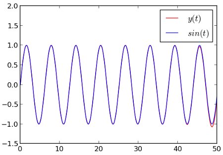
The resulting plot compares our solution (red) with the exact solution (blue). See how our result eventually detaches itself from the actual solution as a consequence of many successive approximations ? As DDEs tend to create chaotic behaviors, you can expect the error to explode very fast. As I am no DDE expert, I would recommend checking for convergence in all cases, i.e. increasing the time resolution and see how it affects the result. Keep in mind that the past values of Y(t) are computed by interpolating the values of Y found at the previous integration points, so the more points you ask for, the more precise your result.
An example with parameters
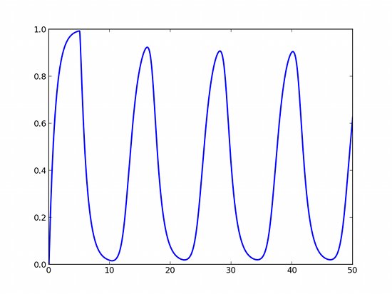
You can set the parameters of your model at integration time, like in Scipy’s ODE and odeint. As an example, imagine a chemical product with degradation rate $r$, and whose production rate is negatively linked to the quantity of this same product at the time $(t-d)$:
We have three parameters that we can choose freely. For $K = 0.1$, $d = 5$, $r = 1$, we obtain oscillations !
1 2 3 4 5 6 7 8 | |
Example with several variables
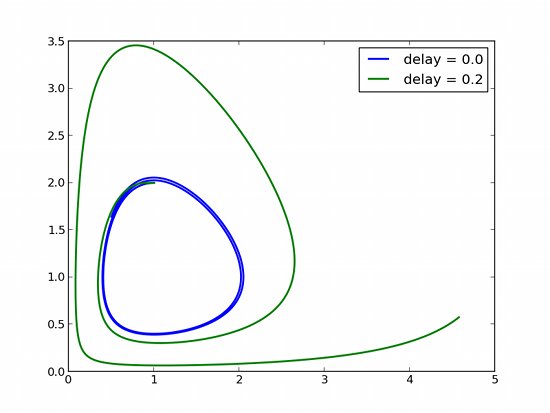
The variable Y can be a vector, which means that you can solve DDE systems of several variables. Here is a version of the famous Lotka-Volterra two-variables system, where we introduce a delay $d$. For $d=0$ the system is a classical Lotka-Volterra system ; for $d\neq 0$ the system undergoes an important amplification:
1 2 3 4 5 6 7 8 9 10 11 12 13 14 | |
Example with a non-constant delay
In this last example the delay depends on the value of $y(t)$ :
1 2 3 4 5 | |
